I attended and presented the following poster. LOCC only holds if one demands that in a classical – quantum connection that QM is not altered.
Archives For November 30, 1999

T C Andersen 2019 J. Phys.: Conf. Ser. 1275 012038 – 9th International Workshop DICE2018 : Spacetime – Matter – Quantum Mechanics
Abstract. The recent experimental proposals by Bose et al. and Marletto et al. (BMV) outline a way to test for the quantum nature of gravity by measuring gravitationally induced differential phase accumulation over the superposed paths of two ∼ 10−14kg masses. These authors outline the expected outcome of these experiments for semi-classical, quantum gravity and collapse models. It is found that both semi-classical and collapse models predict a lack of entanglement in the experimental results. This work predicts the outcome of the BMV experiment in Bohmian trajectory gravity – where classical gravity is assumed to couple to the particle configuration in each Bohmian path, as opposed to semi-classical gravity where gravity couples to the expectation value of the wave function, or of quantized gravity, where the gravitational field is itself in a quantum superposition. In the case of the BMV experiment, Bohmian trajectory gravity predicts that there will be quantum entanglement. This is surprising as the gravitational field is treated classically. A discussion of how Bohmian trajectory gravity can induce quantum entanglement for a non superposed gravitational field is put forward.
This paper is a result of a talk I gave at DICE2018. The trip and the talk allowed me to sharpen the math and the arguments in this paper. I’m convinced that the results of a BMV like experiment would show these results – namely that gravity violates QM! Most physicists are of course on the opposite side of this and would assume that QM would win in a BMV experiment.
For those of the main camp, this paper is still important, as it describes another way to approximate quantum gravity – one that works better than the very often used Rosenfeld style semi-classical gravity. Sitting through talks where researchers use the semi-classical approximation in order to do sophisticated quantum gravity phenomenology has convinced me that often the results would change significantly if they had of used a Bohmian trajectory approach instead. The chemists figured this out a while ago – a Bohmian approximation is much more accurate than semi-classical approximations.
In some sense semi-classical gravity seems more complicated than Bohmian trajectory gravity, as in semi-classical gravity the gravitational field has to somehow integrate the entire position space of the wave function (a non local entity) in real time (via the Schr ̈odinger – Newton equation), in order to continuously use the expectation value as a source for the gravitational field. In Bohmian mechanics, the gravitational field connects directly to an existing ’hidden’ particle position, which is conceptually simpler.

Abstract
An electron model is presented where charge, electromagnetic and quantum effects are generated from pilot wave phenomena. The pilot waves are constructed from nothing more than gravitational effects. First the general model of the electron is proposed. Then the physical consequences are laid out, showing that this model can generate large electron – electron forces, which are then identified with the Coulomb force. Further, quantum mechanical effects are shown to emerge from this model.
Electron model:
An electron is modelled as a small region of space which has a varying mass. The origin of this varying mass will not be discussed here. The mass of the electron is given as
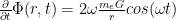
me(t) = me*((1 – f) + f*sin(vt))
where v is some frequency, and f is the proportion of mass that is varying, so f is from 0 –> 1
This varying mass will give rise to very large changes in gravitational potential – essentially the time derivative of the mass will be a potential that has a slope proportional to the frequency. Assume that this frequency is very high, and you can see potential for some huge effects to come into play, as compared with the tiny gravitational field of a normal mass the size of an electron.
Throughout this paper only classical physics will be used, and on top of that, the only field used will be that of gravity (GR).
I said that the mechanism for this time – varying mass will not be discussed, but here are two possibilities. One possibility is that electrons are some sort of wormhole, with some portion of their mass disappearing into and out of this wormhole, like some mass bouncing between two open throats. The other more simple way this could happen is if the electron was simply losing mass off to infinity – and getting it back – in a periodic fashion.
Coulomb Attraction
So how would two of these time varying mass electrons interact?
I will use the 2014 paper “Why bouncing droplets are a pretty good model of quantum mechanics“ as a starting point.
Please open up that paper and have a look:
In section 4.3 – 4.4, the authors use analogy of two vacuum cleaners(!) to come up with a mechanism for an “inverse square force of attraction between the nozzles”.

Where ρ is the density of air and Q is the volume of air flow at each nozzle. I will use this train of thought to come up with a similar inverse square relation for my electron model.
In the equation above, ρ*Q gives the mass intake of one nozzle. In my model ρ*Q is thus the same as time rate of change of the mass of the electron, which averages out to f*me*ν, where
f = fraction of electron mass that is varying (f = 1 – me(min)/me)),
me == rest mass of electron,
and
ν = frequncy (greek nu).
So we have f*me*ν == ρQ, substituting into (8) from Brady and Anderson, we get
dp/dt = f*me*ν/(4πr^2)*Q
Where Q is still some volume flow, in m^3/sec. What, though is the volume flow for an electron – its not sucking up the surrounding air! One possibility is to model Q for my electron model as a spherical surface at some ‘electron radius’, with a speed of light as the velocity. So we have Q = 4πre^2*c and we get the force equation:
dp/dt = f*me*ν*(4πre^2*c)/(4πr^2)
This is the force on an electron nearby another electron at distance r in the model.
This should equal the Coulomb force law: (ke is the coulomb constant)
f*me*ν*(re^2*c)/(r^2) = ke*q*q/r^2
f*me*ν*(re^2*c) = ke*q*q
Now the fraction f, the frequency ν and the re are all unknowns. But lets use the classical electron radius for re, and a fraction f equal to the fine structure constant. Then we get solving numerically for ν the frequency… which is about 1000 times the Compton frequency. (So close to it in some ways)
There are of course other options, as the effective radius of this electron is not known and also the mass fraction is unknown. So this result is more for scale’s sake than anything. Still I will use these numbers for the rest of this paper.
Also interesting is to derive the value of the coulomb force between electrons – simply calculate (leave f alone for now),
f*me*ν*(re^2*c)
This gets to about a factor of 1000 or so away from the correct answer for ke*q*q. But not bad considering that I present no reason why to choose the Compton values for radius and frequency, other than a first jab in the dark.
In section 4.5 – 4.10 the authors show how these pulsating bubbles follow Maxwell’s equations to a good approximation. In the model of the electron presented here, that approximation will be orders of magnitude better across a very large parameter space, as the GR field is much better behaved than bubbles in water, to put it mildly.
Its also easy to see that the resulting model is fully compatible with relativity and GR. Its after all made entirely out of gravity.
Quantum Mechanical Behaviour
The electrons modelled here, which only contain a varying mass, can produce electrical effects that exactly match that of the electric field. As the Brady and Anderson paper continues in part 5, so will we here.
In actual fact, since these electrons have been modelled using the same sort of pilot wave phenomena as Brady and Anderson use, there is not much further to do. QM behaviour erupts from these electron models if you follow sections 5, 6 and 7.
Pilot wave behaviour is outlined in the Brady and Anderson paper.
Conclusion
Electrons made with this model exhibit all the expected forces of electromagnetism, all without introducing electric fields at all. Electrical behaviour is then seen as a phenomena of Gravity, rather than its own field.
These electrons also behave according to the laws of QM, all by generating QM effects using pilot wave mechanics.
From the Brady and Anderson conclusion:
“These results explain why droplets undergo single-slit and double-slit diffraction, tunnelling, Anderson localisation, and other behaviour normally associated with quantum mechanical systems. We make testable predictions for the behaviour of droplets near boundary intrusions, and for an analogue of polarised light.”
This I believe shows a possible way to unify Electro Magnetism, General Relativity, and Quantum Mechanics.
Appendix
There would be much work to do to turn this into a proper theory, with some things needed:
1) What happens with multiple electrons in the same region? A: I think that the linearity of GR in this range assures that the results are the same as EM. It would show a path to finding the limits of EM in areas of high energy, etc.
2) How do protons/quarks work? A: It would seem that quarks might be entities with more complicated ways of breathing mass in and out. This is something that is apparent from their larger actual size, which approaches the maximum size allowed to take part in the geometrical pilot wave, which may run at the compton frequency.
3) Why is charge quantized? A: To me, it seems that the answer to this may be that electrons have quantized charge and protons/quarks are using feedback to keep to the same charge. What about electrons, why are they all the same? I think that’s a puzzle for another day, but perhaps a wormhole model of the electron could be made where the frequency and magnitude of the varying mass would be set from GR considerations.
I don’t expect this model to be instantly accurate, or to answer all questions right away, but the draw to unify EM, QM and Gravity is strong. Any leads should be followed up.
See also
Oza, Harris, Rosales & Bush (2014), Pilot-wave dynamics in a rotating frame MIT site: John W.M. Bush Is quantum mechanics just a special case of classical mechanics? Monopole GR waves Other posts on this site as well..–Tom Andersen
May 17, 2014
How is that even a question?
Previous posts have all not mentioned quantum effects at all. That’s the point – we are building physics from General Relativity, so QM must be a consequence of the theory, right?
Here are some thoughts:
QM seems to not like even special relativity much at all. It is a Newtonian world view theory that has been modified to work in special relativity for the most part, and in General Relativity not at all.
There are obvious holes in QM – the most glaring of which is the perfect linearity and infinitely expandable wave function. Steven Weinberg has posted a paper about a class of QM theories that solve this problem. In essence, the solution is to say that the state vector degrades over time, so that hugely complex, timeless state vectors actually self collapse due to some mechanism. (Please read his version for his views, as my comment are from my point of view.)
If one were to look for a more physical model of QM, something along the lines of Bohm’s hidden variables, then what would we need:
Some sort of varying field that supplies ‘randomness’:
- This is courtesy of the monopole field discussed in previous posts about the proton and the electron.
Some sort of reason for the electron to not spiral into the proton:
- Think De Broglie waves – a ‘macroscopic’ (in comparison to the monopole field) wave interaction. still these waves ‘matter waves’ are closely tied to the waves that control the electromagnetic field.
- Put another way – there is room for many forces in the GR framework, since dissimilar forces ignore each other for the most part.
- Another way of thinking about how you talk about multidimensional information waves (hilbert spaces of millions of dimensions for example), is to note that as long as there is a reasonable mechanism for keeping these information channels separate, then there is a way to do it all with a meta field – GR.
Quantum field theory:
- This monopole field is calculable and finite, unlike the quantum field theories of today, which are off by a factor of 10100 when trying to calculate energy densities, etc.
Re: http://en.wikipedia.org/wiki/Woodward_effect
Now I’m not sure that he is onto something real or not, although experiments are still being performed which detail positive results.
He does have some pretty convincing arguments about what happens to an object with a varying mass:
Let us suppose that, viewed in our inertial frame of reference moving with respect to the brick, when the mass of the brick changes, its velocity changes too so that its momentum remains unchanged. (The cause of the velocity change is mysterious. After all, driving a power fluctuation in the brick to excite a mass fluctuation need not itself exert any net force on the brick. But we’ll let that pass.) We see the brick accelerate. Now we ask what we see when we are located in the rest frame of the brick. The mass fluctuates, but in this frame the brick doesn’t accelerate since its momentum was initially, and remains, zero. This, by the principle of relativity, is physically impossible. If the brick is observed to accelerate in any inertial frame of reference, then it must accelerate in all inertial frames. We thus conclude that mass fluctuations result in violations of local momentum conservation if the principle of relativity is right.
Of course no ‘real’ physicist thinks that you can change the mass of something without a pipe of energy or mass leading into it, but that’s what he means here – some ‘magical’ varying mass. I assume that for my electron model, this varying mass is only a local effect – there is a secret topological ‘wormhole’ pipe that connects two electrons together, so the total mass is constant.
So does Woodwards insight give us any guidance with the effects of the resulting monopole gravitational waves on other varying masses? We can see right away that momentum conservation for such a topological system is only adhered to over a time average.
Look at the diagram from Woodwards article:
http://physics.fullerton.edu/~jimw/nasa-pap/

We see shades of my varying mass model. I am not saying that electrons can self accelerate, but more that the interaction of varying mass objects leads to entirely new physics, without introducing any new equations.
With monopole gravitational waves, the electron will feel a varying force, and the averaged momentum rule from Woodward would then imply that the net average acceleration on the particle is in one direction only, depending on the phase of the arriving wave. Of course these phases are what are called charge – the electron wants to maximize the acceleration, in order to go down the potential energy landscape in the best direction.
Take this size of an electron as the ‘black hole’ size. That is about 10-55 m I think. Then for a solid, we have about 3.35*1028 molecules water per m cubed, h2O, so 7e**29 electrons / m**3 – say 1e30 electrons per cubic metre. With a 1.48494276 × 10⁻²⁷ m / kg conversion constant for the Schwarchild radius of an object measured in kg, and an electron mass of 9.10938291(40)×10−31, we get diameter of 2.6 10-58m, so cross section is 7e-116 and then the total area of a cubic metre of water is about 1e-85 m**2/m
So what is the neutrino cross section.
Say neutrinos only interact with electrons when they hit the actual black hole part. Also assume that neutrinos are much smaller than electrons.
How many meters of water would a ray penetrate before hitting an electron within its -black hole radius?
1e-85 m**2, which works out to a coverage of one part in 1e85, so 1e85 meters would ensure a hit. This is vastly larger than the real distance, which is only a few light years, 1e17 m or so.
So I guess that this idea is very wrong on some counts.
If you use the radius of the electron as a kerr naked ring singularity, you get 1e-37 metres, or 1.616199 × 10⁻³⁵ meters, ie te planck length.
Then with these planck length sized electrons, you get about 1e-70 – which is about 1e-40 m**2/metre of water, still not enough, but closer.
Funny how the kerr radius of an electron mass naked singularity is the planck mass.
Trying a compton size of 2e-12m instead of 2e-56, makes the
I will show with a few simple equations how it could be that electrons and electromagnetic theory can be constructed from GR alone.
1) The electron is some sort of GR knot, wormhole or other ‘thing’, which has one property – its mass is moving from 0 to 2*me in a wave pattern. Well actually, the mass does not have to all b oscillating, it only changes the math slightly.
2) Due to the birkhoff theorem, the gravitational potential at any time is given by the amount of mass inside a certain radius.
3) Due to 2) above, we can use the simple gravitational formula to describe the potential.

This potential exerts a force that depends on the frequency of the varying mass, taking the derivative to get the slope of the potential holding r steady:
With the mass changing, we have monopole graviational waves emanating (and incoming, since the universe is not empty), from such a structure.
The big assumption here is of course the varying mass of the electron. Where does the mass go? The obvious answer is through some sort of wormhole, so perhaps there is another electron somewhere else with the opposite phase of mass. Shades of the Pauli exclusion principle.
There are lots of places on the internet where one can find electron models where the the electron is modeled on some standing wave, which is what this really amounts to, since electrons would have a huge force on them if the incoming and outgoing are not balanced.
History has showed us that all physical theories eventually fail. The failure is always a complete failure in terms of some abstract perfectionist viewpoint, but in reality, the failure only amounts to small corrections. Take for instance gravity. Newton’s theory is absurd – gravity travels instantly, etc. But it is also simple and powerful, it predictions working well enough to put people on the Moon.
Quantum Mechanics, it would seem, has a lot of physicists claiming that ‘this time is different’ – that QM is ‘right’. Nature does play dice. There are certain details of it yet to be worked out, like how to apply it to fully generalized curvy spacetimes, etc.
Lets look at what would happen if it were wrong. Or rather, lets look at one way that it could be wrong.
QM predicts that there are chances for every event happening. I mean in the following way – there is a certain probability for an electron (say) to penetrate some sort of barrier (quantum tunneling). As the barrier is made higher and or wider, the probability of tunneling goes down according to a well defined formula: (see for example this wikipedia article). Now, the formulas for the tunneling probability do not ‘top out’ – there is a really, really tiny chance that even a slowly moving electron could make it through a concrete wall. What if this is wrong? What if there is a limit as to the size of the barrier? Or put another way – what if there is a limit to probability? Another way to look at this is to say that there is a upper limit on the half life of a compound. Of course, just as Newton’s theory holds extremely well for most physics, it may be hard to notice that there is not an unlimited amount of ‘quantum wiggle’ to ‘push’ particles through extremely high barriers.
Steven Weinberg has posted a paper about a class of theories that try to solve the measurement problem in QM by having QM fail. (It fails a little at a time, so we need big messy physics to have the wave collapse). I agree fully with his idea – that we have to modify QM to solve the measurement problem.
 Andersen, T. C. on ORCID